Dimensionality Reduction in Scikit-learn

Dimensionality reduction is a fundamental process in data science and machine learning. It involves reducing the number of features (variables) in a dataset while retaining as much information as possible. This simplification is essential for improving computational efficiency, reducing storage space, and enhancing the performance of machine learning models. In this article, we'll explore key dimensionality reduction techniques and how to implement them using Scikit-learn.

---

1. What is Dimensionality Reduction?

1.1 Definition

Dimensionality reduction refers to the process of reducing the number of input variables in a dataset. This can be achieved through:

• Feature Selection: Selecting a subset of the original features based on some criteria.
• Feature Extraction: Transforming the data into a lower-dimensional space using mathematical transformations.

The primary goal is to simplify the dataset without losing significant information, making it easier to visualize, process, and model.

1.2 Importance of Dimensionality Reduction

• Reducing Complexity: Simplifies models by decreasing the number of features, which can improve model interpretability and reduce overfitting.
• Improving Visualization: High-dimensional data is challenging to visualize. Reducing dimensions to 2D or 3D allows for graphical representation.
• Mitigating the Curse of Dimensionality: In high-dimensional spaces, data becomes sparse, and models may struggle to find patterns. Dimensionality reduction helps alleviate this issue.
• Enhancing Computational Efficiency: Fewer features lead to faster computation times and less memory usage, which is crucial for large datasets.

---

2. Techniques for Dimensionality Reduction

Several techniques can be used for dimensionality reduction. We'll focus on four primary methods available in Scikit-learn.

2.1 Principal Component Analysis (PCA)

info

Principal Component Analysis (PCA) is an unsupervised linear transformation technique that projects data onto a lower-dimensional subspace by maximizing variance.

Visit our Principal Component Analysis article for more information.

How it Works:

1. Standardization: Center and scale the data if features have different units or scales.
2. Covariance Matrix Computation: Calculate the covariance matrix to understand how variables vary together.
3. Eigenvalue Decomposition: Compute the eigenvalues and eigenvectors of the covariance matrix.
4. Sort Eigenvectors: Order the eigenvectors by decreasing eigenvalues to identify principal components.
5. Projection: Transform the data onto the new feature space defined by the top $k$ eigenvectors.

Considerations:

• PCA assumes linear relationships and maximizes variance.
• The principal components are orthogonal (uncorrelated) to each other.
• It's sensitive to the scale of the data; hence, standardization is crucial.

Scikit-learn Implementation Example:

import matplotlib.pyplot as plt
from sklearn.decomposition import PCA
from sklearn.preprocessing import StandardScaler
from sklearn.datasets import load_iris

# Load dataset
data = load_iris()
X = data.data
y = data.target

# Standardize the data
scaler = StandardScaler()
X_scaled = scaler.fit_transform(X)

# Apply PCA
pca = PCA(n_components=2)
X_pca = pca.fit_transform(X_scaled)

# Plot the reduced data
plt.figure(figsize=(8, 5))
for i, target_name in enumerate(data.target_names):
    plt.scatter(X_pca[y == i, 0], X_pca[y == i, 1], label=target_name)

plt.xlabel('Principal Component 1')
plt.ylabel('Principal Component 2')
plt.title('PCA of Iris Dataset')
plt.legend()
plt.show()

Explanation:

• Data Loading:

  • load_iris(): Loads the Iris dataset, which contains 150 samples of iris flowers with four features (sepal length, sepal width, petal length, petal width).
  • X: Feature matrix.
  • y: Target vector (species of iris).

• Standardization:

  • StandardScaler(): Creates an instance of the scaler.
  • X_scaled = scaler.fit_transform(X): Fits the scaler to X and transforms it to have zero mean and unit variance.

• PCA Application:

  • PCA(n_components=2): Initializes PCA to reduce data to two principal components.
    • n_components=2: Number of principal components to keep.
  • X_pca = pca.fit_transform(X_scaled): Fits PCA to the standardized data and transforms it.

• Visualization:

  • The code uses a loop to plot each class separately:

    for i, target_name in enumerate(data.target_names):
        plt.scatter(X_pca[y == i, 0], X_pca[y == i, 1], label=target_name)
    • X_pca[y == i, 0]: Principal Component 1 for class i.
    • X_pca[y == i, 1]: Principal Component 2 for class i.
    • label=target_name: Labels each class with its corresponding species name.
  • plt.legend(): Adds a legend with species names from data.target_names.

Interpretation:

• The scatter plot shows how the samples are distributed in the space of the first two principal components.
• Clusters corresponding to different species indicate that PCA has captured significant variance related to species differentiation.

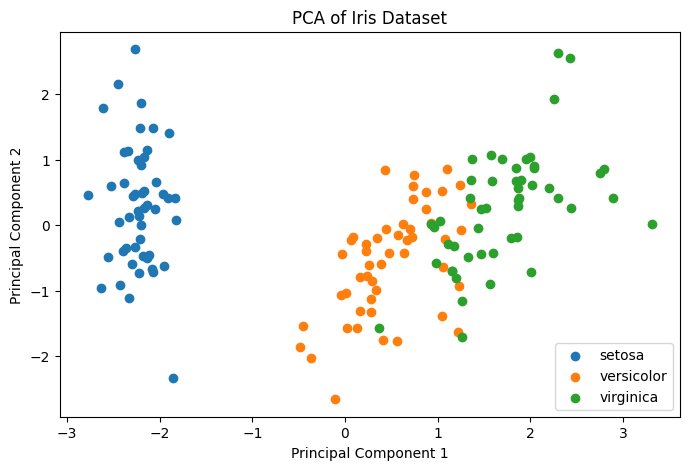
Figure 1: Principal Component Analysis PCA Example.

2.2 Singular Value Decomposition (SVD)

info

Singular Value Decomposition (SVD) is a matrix factorization technique that decomposes a matrix into three other matrices and is particularly useful for sparse or large datasets.

Visit our Singular Value Decomposition article for more information.

How it Works:

1. Matrix Decomposition: Decompose the original data matrix $\mathbf{X}$ into $\mathbf{U \Sigma V}^\top$, where:

   • $\mathbf{U}$: Left singular vectors.
   • $\mathbf{\Sigma}$: Diagonal matrix of singular values.
   • $\mathbf{V}^\top$: Right singular vectors.

2. Dimensionality Reduction: Select the top $k$ singular values and corresponding vectors to approximate the original matrix.

Considerations:

• Effective for data with missing values or when PCA is computationally intensive.
• Unlike PCA, SVD does not require centering the data.

Scikit-learn Implementation Example:

import matplotlib.pyplot as plt
from sklearn.decomposition import TruncatedSVD
from sklearn.datasets import load_digits

# Load dataset
data = load_digits()
X = data.data
y = data.target

# Apply Truncated SVD
svd = TruncatedSVD(n_components=2, random_state=42)
X_svd = svd.fit_transform(X)

# Plot the reduced data
plt.figure(figsize=(8, 5))
scatter = plt.scatter(X_svd[:, 0], X_svd[:, 1], c=y, cmap='viridis', edgecolor='k', s=50)
plt.xlabel('Component 1')
plt.ylabel('Component 2')
plt.title('Truncated SVD of Digits Dataset')
plt.colorbar(scatter, ticks=range(10), label='Digit')
plt.show()

Explanation:

• Data Loading:

  • load_digits(): Loads the Digits dataset with images of handwritten digits.
  • X: Flattened pixel values.
  • y: Labels of the digits.

• Truncated SVD Application:

  • TruncatedSVD(n_components=2, random_state=42): Initializes Truncated SVD for dimensionality reduction.
    • n_components=2: Number of components to keep.
    • random_state=42: Ensures reproducibility.
  • X_svd = svd.fit_transform(X): Fits Truncated SVD to X and transforms it.

• Visualization:

  • plt.scatter(...): Plots the first two SVD components.
    • X_svd[:, 0]: Component 1.
    • X_svd[:, 1]: Component 2.
    • c=y: Colors points based on digit labels.
    • cmap='viridis': Colormap for multiple classes.
    • edgecolor='k': Black edge around points.
    • s=50: Size of the points.
  • plt.colorbar(...): Adds a colorbar indicating digit labels.

Interpretation:

• The scatter plot shows the distribution of digits in the space of the first two SVD components.
• Clusters indicate that Truncated SVD captures important patterns in the data.

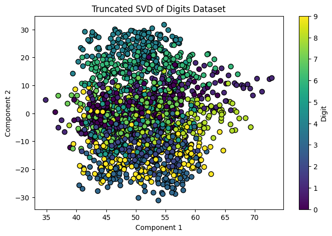
Figure 2: SVD Singular Value Decomposition Example .

tip

Note on PCA vs. TruncatedSVD

While both TruncatedSVD and PCA (Principal Component Analysis) with svd_solver='arpack' can be used for dimensionality reduction, they are not exactly the same.

PCA involves several steps:

1. Centering the Data: Subtracting the mean to center the data around the origin.
2. Computing the Covariance Matrix: Understanding how variables vary together.
3. Eigenvalue Decomposition: Finding eigenvectors and eigenvalues of the covariance matrix.
4. Projection: Projecting the data onto the top eigenvectors.

When using PCA in Scikit-learn with svd_solver='arpack', the ARPACK library computes the SVD of the covariance matrix efficiently.

TruncatedSVD, on the other hand:

• Does Not Center the Data: It works directly on the data without mean subtraction.
• No Covariance Matrix Computation: It performs SVD on the data matrix itself.
• Singular Vectors vs. Eigenvectors: It computes singular vectors of the data matrix, not eigenvectors of the covariance matrix.

Key Differences:

• Centering:
  • PCA centers the data.
  • TruncatedSVD does not center the data.
• Covariance Matrix:
  • PCA computes it.
  • TruncatedSVD skips it.
• Vectors Computed:
  • PCA computes eigenvectors.
  • TruncatedSVD computes singular vectors.

When to Use Each:

• Use PCA when:
  • You need traditional PCA with data centering.
  • You want to analyze the explained variance ratio.
• Use TruncatedSVD when:
  • You're working with sparse data or need efficiency.
  • Data centering is not required or not feasible.

2.3 Linear Discriminant Analysis (LDA)

info

Linear Discriminant Analysis (LDA) is a supervised technique that finds a linear combination of features that best separates two or more classes.

Visit our Linear Discriminant Analysis article for more information.

How it Works:

1. Compute Scatter Matrices:

   • Within-Class Scatter Matrix ($S_W$): Measures the variability within each class.
   • Between-Class Scatter Matrix ($S_B$): Measures the variability between classes.

2. Solve the Generalized Eigenvalue Problem:

   • Find eigenvectors $\mathbf{w}$ that maximize the ratio $\frac{\mathbf{w}^\top S_B \mathbf{w}}{\mathbf{w}^\top S_W \mathbf{w}}$.

3. Select Linear Discriminants:

   • Choose the top $k$ eigenvectors corresponding to the largest eigenvalues.

4. Project Data:

   • Transform the original data onto the new subspace.

Considerations:

• LDA is both a classifier and a dimensionality reduction technique.
• The maximum number of discriminants is $C - 1$, where $C$ is the number of classes.
• Works best when class distributions are Gaussian with equal covariance.

Scikit-learn Implementation Example:

import matplotlib.pyplot as plt
from sklearn.discriminant_analysis import LinearDiscriminantAnalysis
from sklearn.datasets import load_wine

# Load dataset
data = load_wine()
X = data.data
y = data.target

# Apply LDA
lda = LinearDiscriminantAnalysis(n_components=2)
X_lda = lda.fit_transform(X, y)

# Plot the reduced data
plt.figure(figsize=(8, 5))
for i, target_name in enumerate(data.target_names):
    plt.scatter(X_lda[y == i, 0], X_lda[y == i, 1], label=target_name)

plt.xlabel('Linear Discriminant 1')
plt.ylabel('Linear Discriminant 2')
plt.title('LDA of Wine Dataset')
plt.legend()
plt.show()

Explanation:

• Data Loading:

  • load_wine(): Loads the Wine dataset, which includes chemical analysis of wines from three different cultivars.
  • X: Chemical properties of the wines.
  • y: Cultivar labels.

• LDA Application:

  • LinearDiscriminantAnalysis(n_components=2): Initializes LDA to reduce data to two dimensions.
    • n_components=2: Number of linear discriminants to keep (maximum is number of classes - 1).
  • X_lda = lda.fit_transform(X, y): Fits LDA to X and y, and transforms X.

• Visualization:

  • The code uses a loop to plot each class separately:

    for i, target_name in enumerate(data.target_names):
        plt.scatter(X_lda[y == i, 0], X_lda[y == i, 1], label=target_name)
    • X_lda[y == i, 0]: Linear Discriminant 1 for class i.
    • X_lda[y == i, 1]: Linear Discriminant 2 for class i.
    • label=target_name: Labels each class with its corresponding wine cultivar name.
  • plt.legend(): Adds a legend with cultivar names from data.target_names.

Interpretation:

• The scatter plot shows how well LDA separates the three wine classes.
• Clear separation indicates that LDA effectively captures class differences.

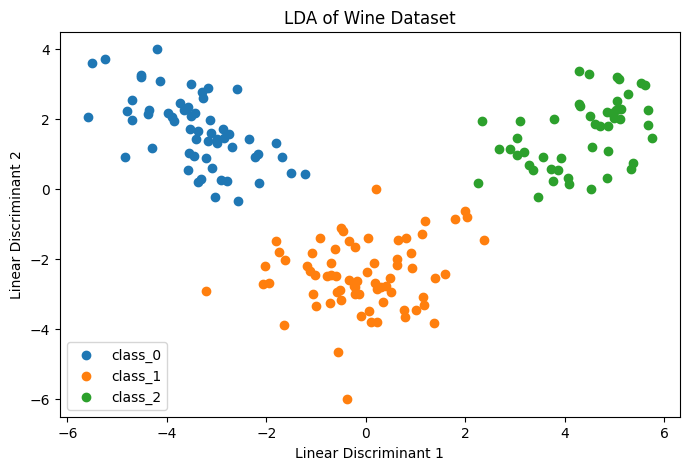
Figure 3: Linear Discriminant Analysis LDA Example.

2.4 Kernel PCA

info

Kernel PCA extends PCA to nonlinear datasets by applying a kernel function, allowing it to capture nonlinear relationships.

Visit our Kernel Principal Component Analysis article for more information.

How it Works:

1. Choose a Kernel Function: Common kernels include Radial Basis Function (RBF), polynomial, and sigmoid.
2. Compute Kernel Matrix: Calculate the kernel matrix $\mathbf{K}$ using the selected kernel.
3. Center the Kernel Matrix: Ensure that the data is centered in the feature space.
4. Eigenvalue Decomposition: Perform eigenvalue decomposition on the kernel matrix.
5. Project Data: Transform the data into the new space using the top $k$ eigenvectors.

Considerations:

• Captures complex, nonlinear structures in the data.
• Choice of kernel and parameters (e.g., gamma in RBF) significantly impacts results.
• Computationally intensive for large datasets.

Scikit-learn Implementation Example:

import matplotlib.pyplot as plt
from sklearn.decomposition import KernelPCA
from sklearn.datasets import make_moons

# Generate dataset
X, y = make_moons(n_samples=200, noise=0.05, random_state=42)

# Apply Kernel PCA
kpca = KernelPCA(n_components=2, kernel='rbf', gamma=15)
X_kpca = kpca.fit_transform(X)

# Plot the reduced data
plt.figure(figsize=(8, 5))
scatter = plt.scatter(X_kpca[:, 0], X_kpca[:, 1], c=y, cmap='coolwarm', edgecolor='k', s=60)
plt.xlabel('Kernel Principal Component 1')
plt.ylabel('Kernel Principal Component 2')
plt.title('Kernel PCA of Moons Dataset')
plt.show()

Explanation:

• Data Generation:

  • make_moons(...): Generates a two-dimensional dataset with a moon-shaped pattern.
    • n_samples=200: Number of samples.
    • noise=0.05: Standard deviation of Gaussian noise.
    • random_state=42: Ensures reproducibility.

• Kernel PCA Application:

  • KernelPCA(n_components=2, kernel='rbf', gamma=15): Initializes Kernel PCA.
    • n_components=2: Number of components to keep.
    • kernel='rbf': Radial Basis Function kernel.
    • gamma=15: Kernel coefficient for RBF.
  • X_kpca = kpca.fit_transform(X): Fits the model to X and transforms it.

• Visualization:

  • plt.scatter(...): Creates a scatter plot of the transformed data.
    • X_kpca[:, 0]: Kernel Principal Component 1.
    • X_kpca[:, 1]: Kernel Principal Component 2.
    • c=y: Colors points based on the generated labels (two classes).
    • cmap='coolwarm': Provides distinct colors for classes.
    • edgecolor='k': Black edge around points.
    • s=60: Size of the points.

Interpretation:

• The scatter plot shows that Kernel PCA successfully unfolds the circular pattern into a linearly separable structure.
• Points from different classes are well-separated in the transformed space.

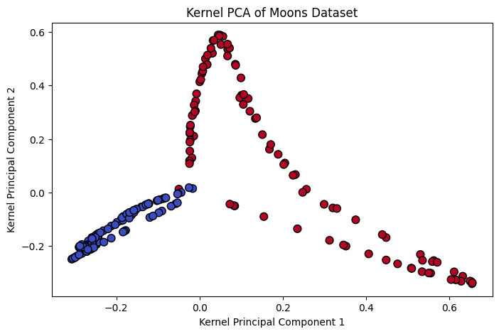
Figure 4: Kernel Principal Component Analysis Example.

2.5 t-Distributed Stochastic Neighbor Embedding (t-SNE)

info

t-Distributed Stochastic Neighbor Embedding (t-SNE) is a nonlinear dimensionality reduction technique primarily used for data visualization. It reduces high-dimensional data to two or three dimensions, making it easier to visualize while preserving the local structure of the data.

Visit our t-Distributed Stochastic Neighbor Embedding article for more information.

How it Works:

1. Compute Pairwise Similarities in High Dimensions:

   • For each pair of data points in high-dimensional space, compute the probability that they are neighbors based on a Gaussian distribution.

2. Compute Pairwise Similarities in Low Dimensions:

   • In the low-dimensional space, compute the probability of similarity between points using a Student's t-distribution with one degree of freedom (Cauchy distribution).

3. Minimize the Kullback-Leibler (KL) Divergence:

   • Optimize the positions of the data points in the low-dimensional space to minimize the KL divergence between the high-dimensional and low-dimensional distributions.

Considerations:

• Computational Intensity: t-SNE is computationally intensive and may not be suitable for very large datasets.
• Hyperparameter Sensitivity: The results can be sensitive to hyperparameters like perplexity and learning rate.
• Non-deterministic Output: Due to random initialization and optimization, results can vary between runs unless a random seed is set.
• Visualization Focus: t-SNE is primarily used for visualization and is not ideal for downstream machine learning tasks.

Scikit-learn Implementation Example:

import matplotlib.pyplot as plt
from sklearn.manifold import TSNE
from sklearn.datasets import load_digits
from sklearn.preprocessing import StandardScaler

# Load dataset
digits = load_digits()
X = digits.data
y = digits.target

# Standardize the data
scaler = StandardScaler()
X_scaled = scaler.fit_transform(X)

# Apply t-SNE
tsne = TSNE(n_components=2, perplexity=30, n_iter=300, random_state=42)
X_tsne = tsne.fit_transform(X_scaled)

# Plot the results
plt.figure(figsize=(10, 7))
scatter = plt.scatter(X_tsne[:, 0], X_tsne[:, 1], c=y, cmap='tab10', edgecolor='k', s=50)
plt.title('t-SNE Visualization of Digits Dataset')
plt.xlabel('t-SNE Feature 1')
plt.ylabel('t-SNE Feature 2')
plt.colorbar(scatter, ticks=range(10), label='Digit')
plt.show()

Explanation:

• Data Loading:

  • load_digits(): Loads the Digits dataset.
  • X: Flattened pixel values of images.
  • y: Digit labels (0-9).

• Standardization:

  • StandardScaler(): Initializes the scaler.
  • X_scaled = scaler.fit_transform(X): Standardizes the data to have zero mean and unit variance.

• t-SNE Application:

  • TSNE(n_components=2, perplexity=30, n_iter=300, random_state=42): Initializes t-SNE.
    • n_components=2: Reduces data to two dimensions.
    • perplexity=30: Balances attention between local and global aspects of the data.
    • n_iter=300: Number of iterations (default is 1,000, but a lower value is used here for speed).
    • random_state=42: Ensures reproducibility.
  • X_tsne = tsne.fit_transform(X_scaled): Fits t-SNE and transforms the data.

• Visualization:

  • plt.scatter(...): Plots the transformed data.
    • X_tsne[:, 0]: t-SNE Feature 1.
    • X_tsne[:, 1]: t-SNE Feature 2.
    • c=y: Colors points based on digit labels.
    • cmap='tab10': Colormap suitable for up to 10 discrete colors.
    • edgecolor='k': Black edge around points.
    • s=50: Size of the points.
  • plt.colorbar(...): Adds a colorbar indicating which color corresponds to which digit.

Interpretation:

• The scatter plot shows clusters corresponding to different digits.
• t-SNE effectively preserves local relationships, making it useful for visualizing high-dimensional data.

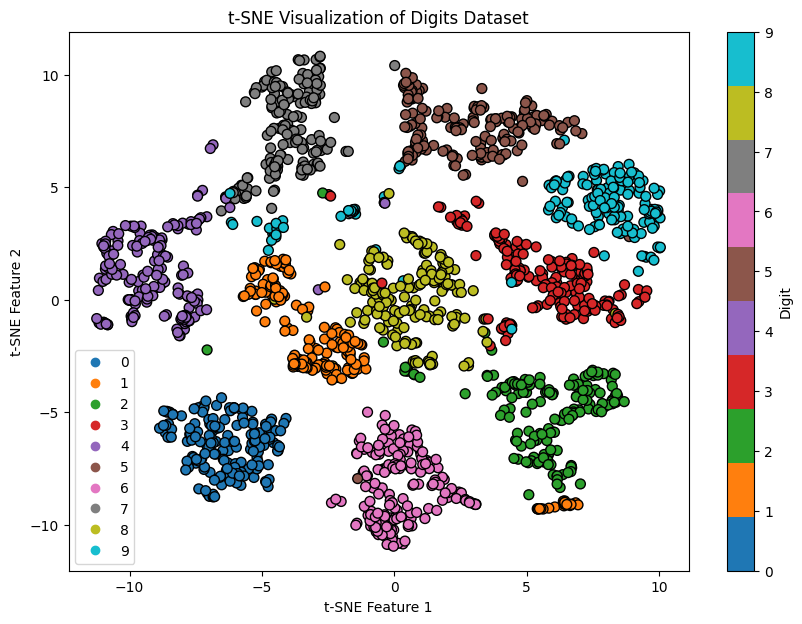
Figure 5: t-Distributed Stochastic Neighbor Embedding Example.

---

3. Practical Considerations

3.1 Choosing the Right Technique

Selecting an appropriate dimensionality reduction method depends on:

• Data Characteristics:

  • Linear vs. Nonlinear: Use PCA or LDA for linear data; Kernel PCA for nonlinear data.
  • Supervised vs. Unsupervised: Use LDA when class labels are available and class separation is desired.

• Purpose:

  • Visualization: PCA and t-SNE are common choices for visualizing high-dimensional data.
  • Preprocessing: PCA and SVD can be used to reduce dimensionality before applying other algorithms.

• Dataset Size:

  • Computational Efficiency: PCA and SVD are efficient for large datasets; Kernel PCA may be slower due to kernel computations.

3.2 Determining the Number of Components

Deciding how many components to keep is crucial.

• Explained Variance Ratio:

  • In PCA, choose $k$ such that the cumulative explained variance reaches a threshold (e.g., 95%).

• Scree Plot:

  • Identify the "elbow" point where adding more components yields diminishing returns.

• Cross-Validation:

  • Evaluate model performance with different numbers of components to find the optimal $k$.

Scikit-learn Implementation Example for Explained Variance:

import numpy as np
import matplotlib.pyplot as plt
from sklearn.decomposition import PCA
from sklearn.preprocessing import StandardScaler
from sklearn.datasets import load_breast_cancer

# Load dataset
data = load_breast_cancer()
X = data.data

# Standardize the data
scaler = StandardScaler()
X_scaled = scaler.fit_transform(X)

# Apply PCA
pca = PCA().fit(X_scaled)
cumulative_variance = np.cumsum(pca.explained_variance_ratio_)

# Plot cumulative explained variance
plt.figure(figsize=(8, 5))
plt.plot(range(1, len(cumulative_variance) + 1), cumulative_variance, marker='o')
plt.title('Cumulative Explained Variance')
plt.xlabel('Number of Components')
plt.ylabel('Cumulative Explained Variance')
plt.axhline(y=0.95, color='r', linestyle='--')
plt.text(10, 0.85, '95% Threshold', color='red', fontsize=12)
plt.show()

Explanation:

• Cumulative Variance Calculation:

  • pca.explained_variance_ratio_: Array of variance ratios for each principal component.
  • np.cumsum(...): Computes the cumulative sum of explained variance.

• Visualization:

  • The plot helps determine how many components are needed to capture a desired amount of variance (e.g., 95%).
  • plt.axhline(...): Draws a horizontal line at 95% cumulative variance.
  • plt.text(...): Places text near the 95% threshold line to indicate the target variance level.

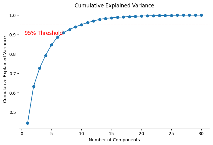
Figure 6: Cumulative Explained Variance Example.

3.3 Interpretation of Components

Interpreting reduced dimensions can be challenging.

• PCA Components:

  • Use pca.components_ to access principal axes and examine feature contributions.
  • Higher absolute values indicate greater influence of a feature on the component.

• LDA Components:

  • Use lda.coef_ to understand the relationship between features and the linear discriminants.

• Limitations:

  • Components are linear combinations of original features and may not have direct physical meaning.

---

4. Best Practices for Dimensionality Reduction

4.1 Standardization Before Applying PCA or LDA

• Why Standardize?

  • Features with larger scales can dominate the principal components.
  • Ensures each feature contributes equally.

• How to Standardize:

  • Use StandardScaler from Scikit-learn.

4.2 Experimentation and Validation

• Try Multiple Techniques:

  • Different methods may yield better results depending on the dataset.

• Cross-Validation:

  • Validate the impact of dimensionality reduction on model performance.

• Visualization:

  • Use plots to assess the effectiveness of dimensionality reduction.

4.3 Combining Techniques

• Hybrid Approaches:

  • Use PCA for initial dimensionality reduction, followed by t-SNE for visualization.

• Feature Engineering:

  • Combine with feature selection methods to enhance model performance.

4.4 Be Mindful of Overfitting

• Avoid Using Test Data:

  • Fit dimensionality reduction models only on training data.

• Pipeline Integration:

  • Use Scikit-learn pipelines to encapsulate preprocessing and modeling steps.

---

5. Conclusion

5.1 Recap of Key Concepts

Dimensionality reduction simplifies complex datasets, making them more manageable for analysis and modeling. Techniques like PCA, SVD, LDA, and Kernel PCA each have their strengths and are suitable for different scenarios.

• PCA: Best for linear, unsupervised dimensionality reduction.
• SVD: Effective for sparse or large datasets.
• LDA: Supervised method maximizing class separation.
• Kernel PCA: Captures nonlinear structures.

Dimensionality reduction is a powerful tool in your data science arsenal. By effectively reducing dimensions, you can improve model performance, enhance visualization, and gain deeper insights into your data.