K-Means vs. other Algorithms
K-Means Clustering is one of the most well-known unsupervised learning algorithms. However, it is not always the best choice for every clustering task. Other algorithms such as DBSCAN, Agglomerative Hierarchical Clustering, Spectral Clustering, and t-SNE have unique strengths that make them more suitable for specific types of datasets. This article provides a detailed comparison of K-Means with these algorithms, helping you understand when to use each method.
1. K-Means vs. DBSCAN (Density-Based Spatial Clustering of Applications with Noise)
Overview of DBSCAN:
DBSCAN is a density-based clustering algorithm that forms clusters by identifying regions of high density separated by regions of lower density. Unlike K-Means, DBSCAN does not require the number of clusters to be specified in advance and can automatically detect clusters of arbitrary shape.
Key Differences:
| Feature | K-Means | DBSCAN |
|---|---|---|
| Cluster Shape | Assumes spherical clusters | Detects clusters of arbitrary shapes |
| Number of Clusters | Must be pre-defined | Automatically detects based on density |
| Handling Noise | Poor handling of noise | Explicitly handles noise (outliers) |
| Distance Metric | Typically uses Euclidean | Uses a distance parameter (ε) to define clusters |
| Scalability | Scales well with large data | Not as scalable for very large datasets |
Example:
- When to use K-Means: Use K-Means when you know the number of clusters, the clusters are roughly spherical, and the data has few outliers.
- When to use DBSCAN: Use DBSCAN when you expect clusters of varying shapes and sizes, and when you want to automatically detect outliers (e.g., in spatial data analysis).
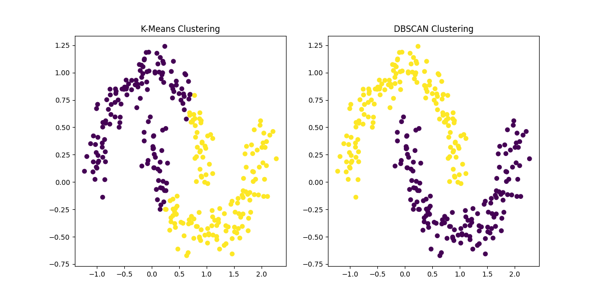
Figure 1: Comparison of K-Means Clustering and DBSCAN on a dataset with two interlocking half-moon shapes. K-Means assumes spherical clusters and struggles to identify the correct clusters, while DBSCAN accurately identifies the non-convex clusters and handles noise.
2. K-Means vs. Agglomerative Hierarchical Clustering
Overview of Agglomerative Hierarchical Clustering:
Agglomerative Hierarchical Clustering is a bottom-up clustering method that builds a hierarchy of clusters by merging or splitting them based on a distance metric. Unlike K-Means, this method does not require the number of clusters to be specified initially.
Key Differences:
| Feature | K-Means | Hierarchical Clustering |
|---|---|---|
| Number of Clusters | Predefined | Can be chosen by cutting the dendrogram |
| Cluster Shape | Assumes spherical clusters | Works with clusters of arbitrary shapes |
| Scalability | More scalable | Computationally expensive for large datasets |
| Distance Metric | Uses Euclidean distance | Can use various distance metrics |
| Cluster Hierarchy | No hierarchy | Builds a hierarchy of clusters (dendrogram) |
Example:
- When to use K-Means: Use K-Means when you need scalable clustering and already know how many clusters to look for.
- When to use Agglomerative Clustering: Use Agglomerative Clustering when the dataset is small to medium-sized, and you are interested in a hierarchy of clusters or cannot determine the number of clusters beforehand.
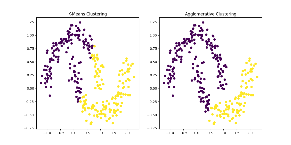
Figure 2: Comparison of K-Means Clustering and Agglomerative Hierarchical Clustering on the same dataset. While K-Means struggles with non-convex shapes, Agglomerative Clustering can detect clusters of arbitrary shapes, although it may be computationally more expensive for larger datasets.
3. K-Means vs. Spectral Clustering
Overview of Spectral Clustering:
Spectral Clustering is a graph-based clustering algorithm that uses the eigenvalues of a similarity matrix to reduce dimensionality before clustering. It is especially useful for detecting clusters with complex structures and shapes that K-Means struggles to identify.
Key Differences:
| Feature | K-Means | Spectral Clustering |
|---|---|---|
| Cluster Shape | Assumes spherical clusters | Handles complex, non-convex clusters |
| Number of Clusters | Must be predefined | Can determine clusters based on eigenvalue gaps |
| Dimensionality | Works in raw data space | Works on reduced dimensionality from eigenvalues |
| Scalability | Highly scalable | Less scalable, requires eigen decomposition |
Example:
- When to use K-Means: Use K-Means for large datasets where clusters are convex and separable in Euclidean space.
- When to use Spectral Clustering: Use Spectral Clustering for complex clustering tasks where the cluster boundaries are non-linear or non-convex, such as image segmentation or graph-based data.
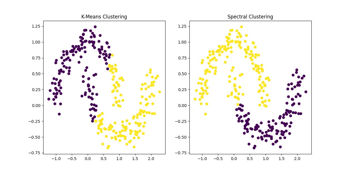
Figure 3: Comparison of K-Means Clustering and Spectral Clustering. Spectral Clustering effectively captures the complex, non-convex shapes in the data that K-Means fails to detect, making it more suitable for datasets with intricate cluster structures.
4. K-Means vs. t-SNE (t-Distributed Stochastic Neighbor Embedding)
Overview of t-SNE:
t-SNE is a dimensionality reduction technique primarily used for visualizing high-dimensional data in a lower-dimensional space (2D or 3D). While not explicitly a clustering algorithm, t-SNE is often used to visualize clusters.
Key Differences:
| Feature | K-Means | t-SNE |
|---|---|---|
| Purpose | Clustering | Visualization |
| Dimensionality | Operates on raw data | Reduces dimensionality for visualization |
| Number of Clusters | Must be predefined | Does not explicitly define clusters |
| Interpretation | Provides hard cluster assignments | Provides a visual map of data relationships |
| Scalability | More scalable | Computationally expensive for large datasets |
Example:
- When to use K-Means: Use K-Means when you need hard cluster assignments for your data.
- When to use t-SNE: Use t-SNE when you want to visualize high-dimensional data and detect patterns visually. t-SNE helps in exploring how data points are related, even though it doesn’t give explicit cluster memberships.
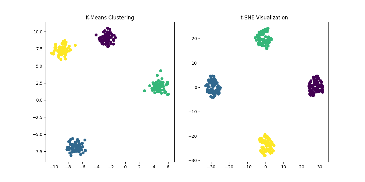
Figure 4: Comparison of K-Means Clustering and t-SNE. While K-Means clusters the data based on predefined centroids, t-SNE provides a low-dimensional representation of the data that helps in visualizing the structure of high-dimensional data.
5. K-Means vs. UMAP (Uniform Manifold Approximation and Projection)
Overview of UMAP:
UMAP is another dimensionality reduction technique that, like t-SNE, is often used for visualizing clusters. It can also be used for non-linear dimensionality reduction, and it is generally faster than t-SNE while preserving more of the global structure in the data.
Key Differences:
| Feature | K-Means | UMAP |
|---|---|---|
| Purpose | Clustering | Dimensionality Reduction & Visualization |
| Dimensionality | Works on raw data | Reduces dimensionality to 2D or 3D |
| Cluster Assignment | Hard clusters | Provides a visual representation of clusters |
| Scalability | Highly scalable | More scalable than t-SNE, but less than K-Means |
Example:
- When to use K-Means: Use K-Means for clustering tasks where the number of clusters and hard cluster assignments are needed.
- When to use UMAP: Use UMAP when you want to reduce high-dimensional data into a low-dimensional space for visualization, particularly when you need to preserve both local and global data structure.
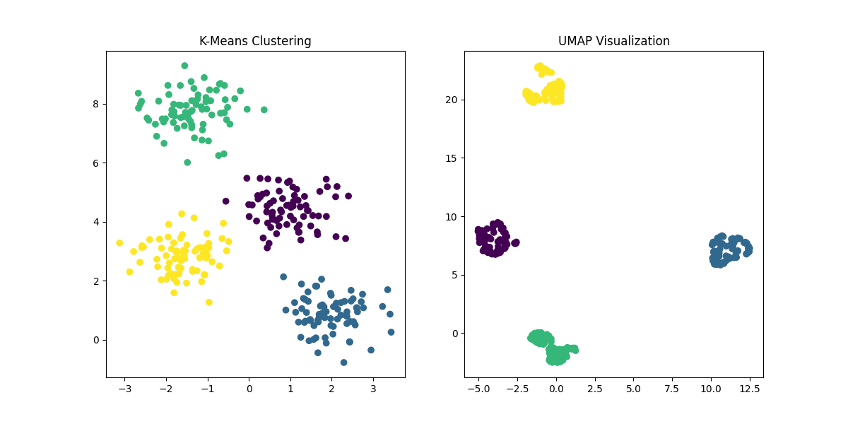
Figure 5: Comparison of K-Means Clustering and UMAP. UMAP, like t-SNE, is used for dimensionality reduction and visualization, preserving more of the global structure compared to t-SNE, and providing an alternative way to explore the data's intrinsic patterns.
Conclusion
K-Means Clustering is a simple and effective algorithm for many clustering tasks, but it is not a one-size-fits-all solution. Depending on your data and use case, alternative algorithms like DBSCAN, Agglomerative Hierarchical Clustering, Spectral Clustering, t-SNE, or UMAP may provide better results.
- Use K-Means: When the number of clusters is known, clusters are spherical, and the dataset is relatively large.
- Use DBSCAN: When clusters have arbitrary shapes and you want to detect noise or outliers.
- Use Agglomerative Clustering: When you need hierarchical relationships or cannot pre-define the number of clusters.
- Use Spectral Clustering: When clusters have complex, non-convex shapes, or in graph-based data.
- Use t-SNE/UMAP: When you need to visualize high-dimensional data and explore relationships in a lower-dimensional space.
Each of these algorithms has strengths and weaknesses, and the choice depends on the nature of your data and your specific goals. Understanding the key differences between these methods will help you select the best algorithm for your project.