Descriptive Statistics

Descriptive statistics are fundamental for summarizing and understanding the essential characteristics of a dataset. By employing various statistical measures, we can describe the central tendency, dispersion, and overall shape of the data distribution. This article delves into these concepts in detail, providing the necessary tools to interpret and analyze data effectively.

Measures of Central Tendency

Central tendency measures provide insight into where the center of a dataset lies. They include the mean, median, and mode, each of which offers a different perspective on the data.

1. Mean

The mean is the arithmetic average of a dataset and is calculated by summing all the data points and dividing by the number of points. It is a widely used measure of central tendency, but it can be sensitive to outliers.

$$\text{Mean} (\mu) = \frac{1}{N} \sum_{i=1}^{N} x_i$$

Example: Consider the dataset $X = \{48, 52, 49, 50, 51, 53, 47, 55, 49\}$. The mean is calculated as follows:

• The sum of the data points is $48 + 52 + 49 + 50 + 51 + 53 + 47 + 55 + 49 = 454$.
• The number of data points, $N$, is 9.

The mean is:

$$\mu = \frac{454}{9} \approx 50.44$$

The mean provides a general idea of the data's central value, but if the dataset included a very large or small outlier, the mean could be misleading.

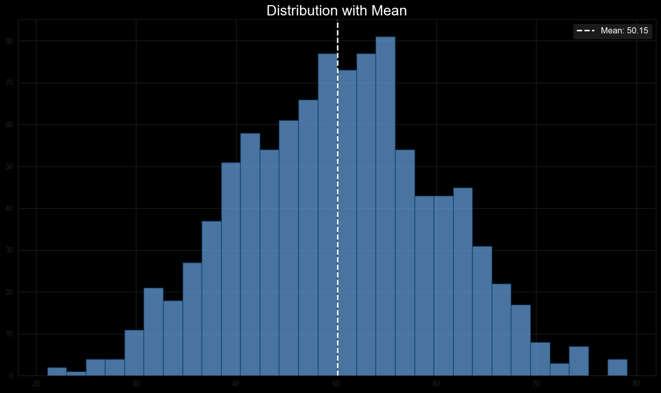
Figure 1: Mean Distribution showing a normal distribution curve with a mean marked by a vertical dashed line.

---

2. Median

The median is the middle value of a dataset when it is ordered from smallest to largest. It is a robust measure of central tendency, particularly in skewed distributions, because it is not affected by outliers.

For a dataset $X = \{x_1, x_2, \dots, x_N\}$, sorted in ascending order:

• If $N$ is odd, the median is $x_{\frac{N+1}{2}}$.
• If $N$ is even, the median is the average of the two middle values: $\frac{x_{\frac{N}{2}} + x_{\frac{N}{2} + 1}}{2}$.

Example

Example: Suppose we have a dataset generated from a normal distribution centered around 50. The median of this dataset would be approximately $49.93$, as shown in the histogram below.

The dataset is modeled after a typical normal distribution, and the median represents the middle value when the data points are ordered. The median value is marked by a vertical dashed line in the histogram.

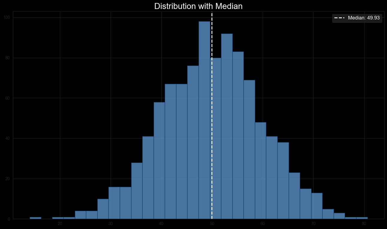
Figure 2: Median Distribution showing a normal distribution curve with the median marked by a vertical dashed line.

---

3. Mode

The mode is the value that appears most frequently in a dataset. A dataset can be:

• Unimodal: Having one mode.
• Bimodal: Having two modes.
• Multimodal: Having more than two modes.
• No mode: If no value repeats.

In the context of a bimodal distribution, the dataset has two distinct peaks, each representing a mode.

---

Example: Consider a dataset that is bimodal, meaning it has two modes. If the dataset is (X = {50, 53, 57, 60, 63, 65}), the modes represent the most frequently occurring values in the dataset. In this example, the dataset shows two distinct peaks at approximately 50 and 60.

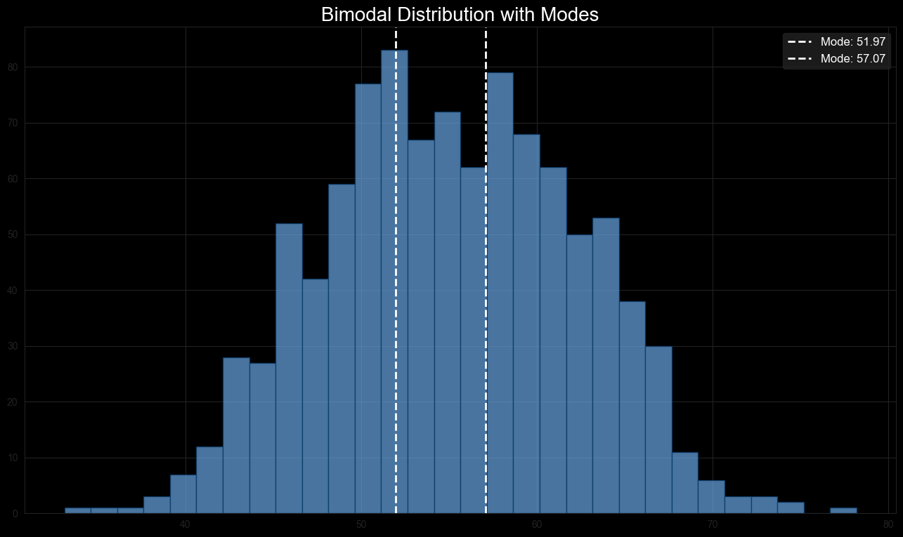
Figure 3: Mode Distribution showing a bimodal distribution, with the modes at approximately 50 and 60, marked by vertical dashed lines.

---

Measures of Dispersion

While measures of central tendency provide insights into the data’s center, measures of dispersion describe the spread of the data. These include range, variance, and standard deviation.

1. Range

The range is the simplest measure of dispersion and is calculated as the difference between the maximum and minimum values in a dataset.

$$\text{Range} = x_{\text{max}} - x_{\text{min}}$$

Example: For the dataset $X = \{3, 7, 8, 5, 12, 14, 21, 13, 18\}$, the range is:

$$\text{Range} = 21 - 3 = 18$$

The range provides a quick sense of the spread of the data but is highly sensitive to outliers.

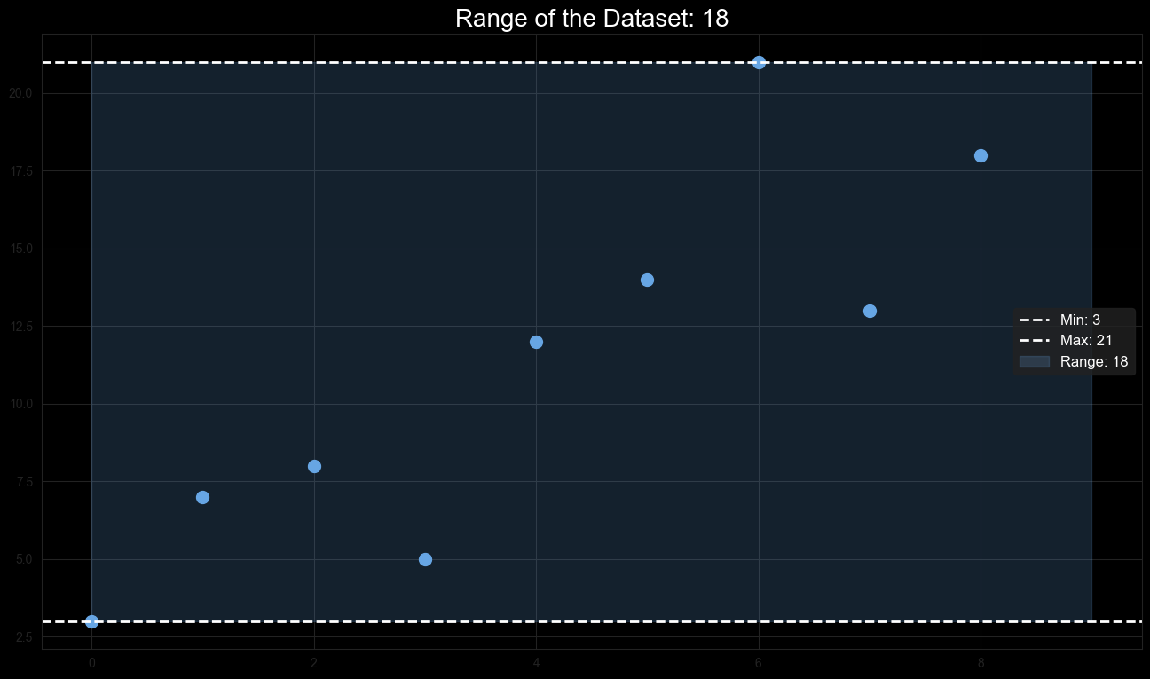
Figure 4: Range Visualization showing the minimum and maximum values, with a shaded area representing the range.

2. Variance

Variance measures how far each data point is from the mean and thus provides a measure of the data's overall spread. It is particularly useful for datasets where the values deviate significantly from the mean.

For a population:

$$\text{Variance} (\sigma^2) = \frac{1}{N} \sum_{i=1}^{N} (x_i - \mu)^2$$

For a sample:

$$\text{Sample Variance} (s^2) = \frac{1}{N-1} \sum_{i=1}^{N} (x_i - \bar{x})^2$$

Where:

• $\mu$ is the population mean.
• $\bar{x}$ is the sample mean.
• $N$ is the number of data points.

Example: Consider the sample dataset $X = \{3, 7, 8, 5, 12\}$.

• The mean $\bar{x}$ is $\frac{3+7+8+5+12}{5} = 7$.
• The squared deviations from the mean are $(3-7)^2 = 16$, $(7-7)^2 = 0$, $(8-7)^2 = 1$, $(5-7)^2 = 4$, and $(12-7)^2 = 25$.

The sample variance is:

$$s^2 = \frac{16 + 0 + 1 + 4 + 25}{5-1} = \frac{46}{4} = 11.5$$

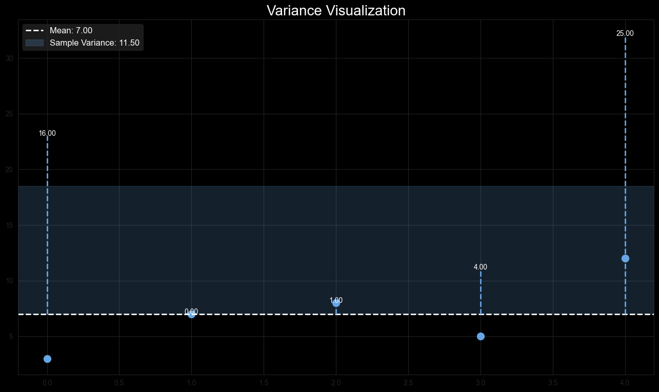
Figure 5: Variance Visualization showing the squared deviations from the mean.

3. Standard Deviation

The standard deviation is the square root of the variance, providing a measure of the average distance from the mean. It is in the same units as the data, making it more interpretable than variance.

For a population:

$$\text{Standard Deviation} (\sigma) = \sqrt{\frac{1}{N} \sum_{i=1}^{N} (x_i - \mu)^2}$$

For a sample:

$$\text{Sample Standard Deviation} (s) = \sqrt{\frac{1}{N-1} \sum_{i=1}^{N} (x_i - \bar{x})^2}$$

Example: Using the sample variance calculated above ($s^2 = 11.5$), the standard deviation is:

$$s = \sqrt{11.5} \approx 3.39$$

Standard deviation provides an understanding of how spread out the data points are from the mean. A higher standard deviation indicates greater variability.

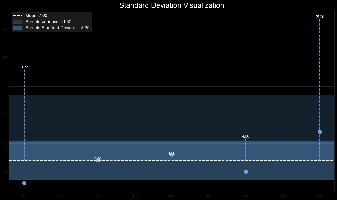
Figure 6: Standard Deviation Visualization showing the standard deviation as a shaded area around the mean.

Importance of Descriptive Statistics

Descriptive statistics are crucial for summarizing large datasets and identifying patterns. They provide the foundation for further statistical analysis and decision-making processes. By understanding the central tendency, dispersion, skewness, and kurtosis, you can gain valuable insights into the data before applying more complex analytical techniques.

Applications in Data Science

• Data Exploration: Descriptive statistics are the first step in exploring and understanding the dataset.
• Data Cleaning: Identifying outliers and unusual patterns helps in cleaning the data.
• Feature Engineering: Insights gained from descriptive statistics can guide the creation of new features in a dataset.

Conclusion

Descriptive statistics are indispensable tools in data analysis, providing a summary of the data's key characteristics. By mastering these concepts, you’ll be better equipped to analyze, interpret, and communicate your findings, laying the groundwork for more advanced statistical techniques.