Probability Theory Basics

Probability theory is a fundamental aspect of statistics and data science, providing the mathematical framework to quantify uncertainty and make predictions based on data. This article delves into the core concepts of probability theory, exploring the nature of probability, independent and dependent events, conditional probability, and Bayes' Theorem.

What is Probability?

Probability is a measure of the likelihood that a particular event will occur. It quantifies uncertainty and is expressed as a number between 0 and 1:

• 0 indicates an impossible event.
• 1 indicates a certain event.

The probability of an event $A$ is denoted by $P(A)$, and it is calculated as:

$$P(A) = \frac{\text{Number of favorable outcomes}}{\text{Total number of possible outcomes}}$$

Example: Rolling a Die

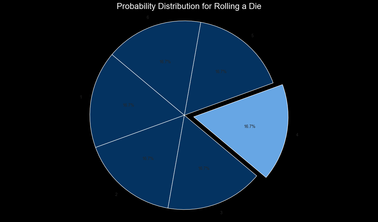
Consider rolling a fair six-sided die. The probability of rolling a 4 (event $A$) is:

$$P(A) = \frac{1}{6} \approx 0.167$$

Since there is one favorable outcome (rolling a 4) out of six possible outcomes (1, 2, 3, 4, 5, 6), the probability of rolling a 4 is approximately 0.167.

Figure 1: Probability Distribution for Rolling a Die, highlighting the probability of rolling a 4.

Independent and Dependent Events

Events can be categorized as independent or dependent based on whether the occurrence of one event affects the probability of another.

1. Independent Events

Independent events are events where the occurrence of one event does not affect the probability of the other. The probability of two independent events $A$ and $B$ occurring together is the product of their individual probabilities:

$$P(A \cap B) = P(A) \times P(B)$$

Example: Tossing Two Coins

When tossing two fair coins, the outcome of the first toss does not affect the outcome of the second toss. If $A$ is the event of getting a heads on the first toss and $B$ is the event of getting a heads on the second toss:

$$P(A) = \frac{1}{2}, \quad P(B) = \frac{1}{2}$$

The probability of getting heads on both tosses (event $A \cap B$) is:

$$P(A \cap B) = \frac{1}{2} \times \frac{1}{2} = \frac{1}{4} = 0.25$$

2. Dependent Events

Dependent events are events where the occurrence of one event affects the probability of the other. The probability of two dependent events $A$ and $B$ occurring together is calculated using conditional probability.

Example: Drawing Cards Without Replacement

Consider drawing two cards from a deck without replacement. If $A$ is the event of drawing an Ace on the first draw and $B$ is the event of drawing an Ace on the second draw, the events are dependent.

• Probability of drawing an Ace first: $P(A) = \frac{4}{52}$
• Probability of drawing an Ace on the second draw, given that an Ace was drawn first: $P(B|A) = \frac{3}{51}$

The probability of both events occurring is:

$$P(A \cap B) = P(A) \times P(B|A) = \frac{4}{52} \times \frac{3}{51} \approx 0.0045$$

Conditional Probability

Conditional probability is the probability of an event occurring given that another event has already occurred. It is denoted by $P(A|B)$ and is calculated as:

$$P(A|B) = \frac{P(A \cap B)}{P(B)}$$

Where:

• $P(A \cap B)$ is the probability of both events $A$ and $B$ occurring.
• $P(B)$ is the probability of event $B$ occurring.

Example: Probability of Drawing a Red Card Given an Ace

Consider a standard deck of 52 cards. Let $A$ be the event of drawing a red card, and $B$ be the event of drawing an Ace.

• $P(A \cap B) = \frac{2}{52}$ (since there are 2 red Aces in a deck).
• $P(B) = \frac{4}{52}$ (since there are 4 Aces in a deck).

The conditional probability of drawing a red card given that an Ace is drawn is:

$$P(A|B) = \frac{\frac{2}{52}}{\frac{4}{52}} = \frac{2}{4} = 0.5$$

This result shows that if an Ace is drawn, there is a 50% chance it is a red Ace.

Bayes' Theorem

Bayes' Theorem is a powerful tool in probability theory that allows us to update our beliefs based on new evidence. It relates the conditional probability of events $A$ and $B$:

$$P(A|B) = \frac{P(B|A) \times P(A)}{P(B)}$$

Where:

• $P(A|B)$ is the posterior probability of $A$ given $B$.
• $P(B|A)$ is the likelihood of $B$ given $A$.
• $P(A)$ is the prior probability of $A$.
• $P(B)$ is the marginal probability of $B$.

Example: Medical Testing

Suppose a diagnostic test for a disease has the following characteristics:

• Sensitivity (true positive rate) = $P(\text{Positive Test}|\text{Disease}) = 0.99$
• Specificity (true negative rate) = $P(\text{Negative Test}|\text{No Disease}) = 0.95$
• Prevalence of the disease in the population = $P(\text{Disease}) = 0.01$

If a person tests positive, what is the probability they actually have the disease?

Using Bayes' Theorem:

$$P(\text{Disease}|\text{Positive Test}) = \frac{P(\text{Positive Test}|\text{Disease}) \times P(\text{Disease})}{P(\text{Positive Test})}$$

Where $P(\text{Positive Test})$ is calculated as:

$$P(\text{Positive Test}) = P(\text{Positive Test}|\text{Disease}) \times P(\text{Disease}) + P(\text{Positive Test}|\text{No Disease}) \times P(\text{No Disease})$$

Substitute the values:

$$P(\text{Positive Test}) = (0.99 \times 0.01) + (0.05 \times 0.99) = 0.0099 + 0.0495 = 0.0594$$

Finally, calculate the posterior probability:

$$P(\text{Disease}|\text{Positive Test}) = \frac{0.99 \times 0.01}{0.0594} \approx 0.167$$

This result indicates that despite a positive test result, there is only a 16.7% chance that the person actually has the disease, emphasizing the importance of understanding and applying Bayes' Theorem in medical testing and other areas.

Law of Total Probability

The Law of Total Probability is used to calculate the probability of an event based on multiple, mutually exclusive scenarios that cover all possible outcomes. If events $B_1, B_2, \dots, B_n$ are mutually exclusive and exhaustive, then for any event $A$:

$$P(A) = \sum_{i=1}^{n} P(A|B_i) \times P(B_i)$$

Example: Probability of Rain Based on Weather Forecasts

Suppose the probability of rain depends on three different weather forecasts:

• $P(\text{Rain}|\text{Forecast 1}) = 0.8$
• $P(\text{Rain}|\text{Forecast 2}) = 0.6$
• $P(\text{Rain}|\text{Forecast 3}) = 0.4$

And the probabilities of each forecast being accurate are:

• $P(\text{Forecast 1}) = 0.5$
• $P(\text{Forecast 2}) = 0.3$
• $P(\text{Forecast 3}) = 0.2$

Using the Law of Total Probability, the overall probability of rain is:

$$P(\text{Rain}) = (0.8 \times 0.5) + (0.6 \times 0.3) + (0.4 \times 0.2) = 0.4 + 0.18 + 0.08 = 0.66$$

There is a 66% chance of rain based on the combined accuracy of the forecasts.

Conclusion

Understanding the basics of probability theory is crucial for data science, as it lays the groundwork for statistical inference, machine learning, and decision-making under uncertainty. By mastering concepts such as independent and dependent events, conditional probability, and Bayes' Theorem, you can make more informed decisions based on data.